- Published on
Sorting Algorithms
- Authors
- Name
- Sriharsha Mopidevi
- Github
- @sriharshamvs
Introduction
A sorting algorithm is an algorithm that puts elements of a list into an order. The most frequently used orders are numerical order and lexicographical order, and either ascending or descending. Sorting is also often useful for producing human-readable output.
Let's look at some terminology before diving into the sorting alogrithms.
Time and Space Complexities
Time Complexity
Time complexity refers to the time taken by an algorithm to complete its execution with respect to the size of the input. Using asymptotic analysis, we can very well conclude the best case, average case, and worst case scenario of an algorithm.
It can be represented in different forms:
Big-O (Ο) − Maximum time required for program execution or Worst Case.
Theta (θ) − Average time required for program execution or Average Case.
Omega (Ω) − Minimum time required for program execution or Best Case.
Space Complexity:
Space complexity refers to the total amount of memory used by the algorithm for a complete execution. It includes both the auxiliary memory and the input.
The auxiliary memory is the additional space occupied by the algorithm apart from the input data. Usually, auxiliary memory is considered for calculating the space complexity of an algorithm.
Their complexities can also be represented in Asymptotic notations(O, θ, Ω).
In Place Sorting
An in-place sorting algorithm uses constant space for producing the output. It sorts the list only by modifying the order of the elements within the list.
It's Space Complexity will be O(1) that is constant space.
Stability of Sorting Algorithm
A sorting algorithm is considered stable if the two or more items with the same value maintain the same relative positions even after sorting.
Now enough with the terminologies. Let's look the first alogrithm.
Bubble Sort
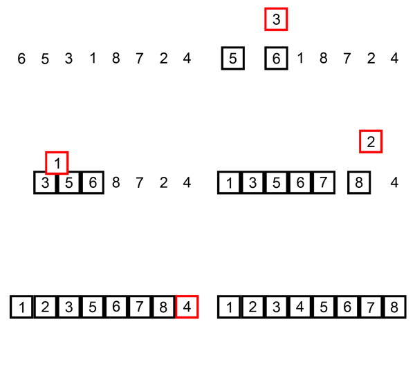
A sorting alogrithm that compares two adjacent elements and swaps them until they are in the intended order.

Code
def bubbleSort(array):
    for i in range(len(array)):
        swapped = False
        for j in range(0, len(array) - i - 1):
            if array[j] > array[j + 1]:
                array[j], array[j+1] = array[j+1], array[j]
                swapped = True
            if not swapped:
                break
Bubble Sort Complexity
| Time Complexity | |
|---|---|
| Best | O(n) |
| Worst | O(n2) |
| Average | O(n2) |
| Space Complexity | O(1) |
| Stability | Yes |
Selection Sort
A sorting algorithm that selects the smallest element from an unsorted list in each iteration and places that element at the beginning of the unsorted list.

Code
for i in range(len(A)):
    idx_min = i
    for j in range(i+1, len(A)):
        if A[idx_min] > A[j]:
            idx_min = j

    A[i], A[idx_min] = A[idx_min], A[i]
Selection Sort Complexity
| Time Complexity | |
|---|---|
| Best | O(n2) |
| Worst | O(n2) |
| Average | O(n2) |
| Space Complexity | O(1) |
| Stability | No |
Insertion Sort
A sorting alogrithm that builds the final sorted array (or list) one item at a time by comparisons.

Code
for i in range(1, len(A)):
    min_value = A[i]
    j = i - 1
    while j>=0 and min_value < A[j]:
        A[j+1] = A[j]
        j = j - 1
    A[j+1] = min_value
Insertion Sort Complexity
| Time Complexity | |
|---|---|
| Best | O(n) |
| Worst | O(n2) |
| Average | O(n2) |
| Space Complexity | O(1) |
| Stability | Yes |
Merge Sort
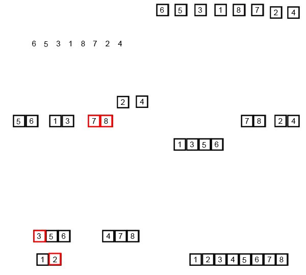
A sorting algorithm that implements divide-and-conquer technique.
- Divide the unsorted list into n sublists, each containing one element (a list of one element is considered sorted).
- Repeatedly merge sublists to produce new sorted sublists until there is only one sublist remaining. This will be the sorted list.

Pseudocode
MergeSort(A, p, r):
    if p > r
        return
    q = (p+r)/2
    mergeSort(A, p, q)
    mergeSort(A, q+1, r)
    merge(A, p, q, r)
Code
def mergeSort(array):
    if len(array) > 1:
        mid = len(array)//2
        left_array = array[:mid]
        right_array = array[mid:]

        mergeSort(left_array)
        mergeSort(right_array)

        i = j = k = 0

        while i < len(left_array) and j < len(right_array):
            if left_array[i] < right_array[j]:
                array[k] = left_array[i]
                i += 1
            else:
                array[k] = right_array[j]
                j += 1
            k += 1

        while i < len(left_array):
            array[k] = left_array[i]
            i += 1
            k += 1

        while j < len(right_array):
            array[k] = right_array[j]
            j += 1
            k += 1
Merge Sort Complexity
| Time Complexity | |
|---|---|
| Best | O(n*log n) |
| Worst | O(n*log n) |
| Average | O(n*log n) |
| Space Complexity | O(n) |
| Stability | Yes |
Quick Sort
Quicksort is a divide-and-conquer algorithm. It works by selecting a 'pivot' element from the array and partitioning the other elements into two sub-arrays, according to whether they are less than or greater than the pivot.
The sub-arrays are then sorted recursively. This can be done in-place, requiring small additional amounts of memory to perform the sorting.

Pseudocode
Pseudocode Quick Sort
quickSort(a[], low, high) {
    if (low < high) {
        pi = partition(arr, low, high);
        quickSort(a, low, pi - 1);  // Left of partition
        quickSort(a, pi + 1, high); // Right to partition
    }
}
Partition Code
partition (a[], low, high) {
    pivot = a[high];
    i = (low - 1)
    for (j = low; j <= high - 1; j++){
        if (a[j] < pivot){
            i++;
            swap(a[i], a[j])
        }
    }
    swap(a[i + 1], a[high])
    return (i + 1)
}
Quicksort Code
def partition(a, low, high):
    pivot = a[high]
    i = low - 1
    for j in range(low, high):
        if a[j] <= pivot:
            i = i + 1
            (a[i], a[j]) = (a[j], a[i])
    (a[i + 1], a[high]) = (a[high], a[i + 1])
    return i + 1

def quickSort(a, low, high):
    if low < high:
        pi = partition(a, low, high)
        quickSort(a, low, pi - 1)
        quickSort(a, pi + 1, high)
Quick Sort Complexity
| Time Complexity | |
|---|---|
| Best | O(n*log n) |
| Worst | O(n2) |
| Average | O(n*log n) |
| Space Complexity | O(log n) |
| Stability | No |
Sources
- Wikipedia
- Programiz
- GeeksforGeeks